In this assignment you will be working extensively with Microsoft Excel 2000
in order to practice spreadsheet skills. For this assignment, assume you have
successfully secured one of the jobs for which you applied in
Create a new folder named Assign4 on your floppy diskette. All of your work for this assignment should be saved in this folder.
Using anonymous FTP, get the text file named cars.csv from the /pub/cs401h path on the computer named cs.unh.edu and store this file in your Assign4 folder.
Open this file with Excel and save the resulting Excel document as a workbook named cars.xls.
Rename the single worksheet in the workbook to “Comparison” and insert a new worksheet before it named “Budget.” Build and format the contents of this Budget worksheet to match the example below:

On the Budget worksheet, define a unique name for each cell that contains a numeric value in the sample above. Use these defined names whenever you reference a cell in any formula on this worksheet. The values circled in red in the sample need to be calculated with formulas. All of the other values should be entered as constants. The math in the formulas is very simple. The only remotely tricky formula is the one that calculates the maximum loan amount. For this formula, you will need to use Excel’s PV function. Look this function up in Excel’s online help and read the description to learn how to use it.
Now, return to the Comparison worksheet and complete it to match the following example:

You will need to enter several formulas to complete this worksheet. Where these formulas need to refer to cells in the Budget worksheet, use the defined names for those cells. Where these formulas need to refer to cells elsewhere on the Comparison worksheet, use standard relative or absolute references as appropriate. A brief description of each formula follows:
- Total MSRP
- The sum of the Base MSRP and the MSRP of Options
- Total Invoice
- The sum of the Base Invoice and the Invoice of Options
- Target Price
- The average of the Total Invoice (plus the Destination Charge) and the Total MSRP
- Loan Required
- The difference of the Target Price and the Available Down Payment (on the Budget worksheet)
- Loan Payment
- Calculated loan payment based upon Loan Required, Annual Interest Rate on Loan, and Term of Loan
- Gas Expense
- Calculated from City Mileage and Highway Mileage based upon number of city and highway miles driven per month
- Estimated Insurance
- Use $500 plus 5% of the Base MSRP as a rough estimate of the ANNUAL insurance cost and calculate a monthly cost from that
- Total Monthly Cost
- The sum of Loan Payment, Gas Expense, and Estimated Insurance
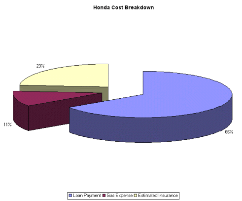
Create a chartsheet named “Honda” that contains a pie chart that demonstrates the relative contributions to the Total Monthly Cost of the Honda CR-V. Your chart should match the following example:

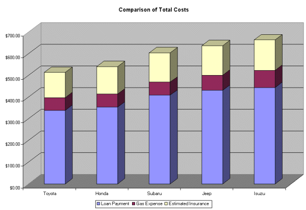
Next, create a chartsheet named “Costs” that contains a stacked bar chart comparing the Total Monthly Costs of all five vehicles and demonstrating the relative components of each total cost. Your chart should match the following example (Hint: if all of your bars are the same height, you’ve probably selected the wrong chart type!):

Insert a new worksheet named “Payments” into your workbook. Assume you’ve decided to buy the Honda CR-V. On the Payments worksheet, create an amortization table that lists every payment you will make on your car loan. The first and last few rows of this table are shown in the sample below. Note that the skip from number 5 to 45 is simply to save space in the sample; your worksheet should include all 49 rows of the table. Use this sample as the basis for constructing your worksheet:

Define names for the appropriate cells in your Comparison worksheet and use these names to bring the Loan Amount and Monthly Payment into your Payment Table. You will also find it worthwhile to explore the Series... option in the Fill submenu under the Edit menu; this will save you a bunch of typing in the first two columns. To calculate the portion of each payment that is interest, use the IPMT function. The other formulas are straightforward.
Select the range of cells with the corners marked in red in the above sample and define it to have the name “Payments.” This will enable you to use this portion of the Payments worksheet as a lookup table.
Add another new worksheet to your workbook and name it “Info.” Using the VLOOKUP function and the Payments range as your lookup table, build this worksheet to match the following example:

The only constant value in this worksheet (other than the text labels, of course) is the value of Today’s Date. When you change this value, the other numeric values should automatically update to reflect the last payment made as of Today’s Date.
Go back through each worksheet and chartsheet in your workbook and give each one a footer that contains your name and a header that contains the date and time of printing. Then, print two copies of each worksheet. The first copy should be in portrait orientation and should display the results of the formulas. The second copy should be in landscape orientation and should display the formulas themselves. When printing the formulas, make sure the column widths are wide enough to display each formula in its entirety before printing. Print one copy of each chartsheet.
Submit your printouts and your diskette.